Derivative Pricing – Semi-Analytic
Lattice Integrator Approaches
1. Introduction
[this page | pdf | references | back links]
Return
to Abstract and Contents
Next
page
1.1 The price of
a (European-style) derivative can be calculated as the discounted expected
value of its payout function, where the expectation is carried out using the
risk-neutral probability distribution. If the payout function and the
risk-neutral probability distribution are both simple functions then the price
of the derivative may be derivable analytically. For example, the Black-Scholes
formulae can be derived analytically (see e.g. Black-Scholes
derivation as the limit of a binomial tree or Black-Scholes
derivation using stochastic calculus). The hedging parameters, i.e. greeks,
applicable to the derivative may also be analytically tractable (see e.g. hedging parameters
applicable to vanilla and binary puts and calls in a Black-Scholes world).
However, for more complicated pay-offs or more complicated risk neutral
probability distributions it is usually not possible to derive equivalent
analytical formulae.
1.2 The most
common approach used to circumvent this problem is to use numerical approaches
such as binomial or trinomial trees that converge to the correct price or other
hedging parameter as the tree becomes more and more finely grained.
Unfortunately, these algorithms are not usually very good at handling
singularities in derivative payout functions. These singularities can arise
directly in the payout function, e.g. payout functions applicable to digital
options have discontinuities at the strike price. They can also arise via
discontinuous first partial derivatives with respect to the underlying (price)
process. These are more common. For example, the first derivative of the payout
function of a vanilla call option is discontinuous at the strike price because
the payoff function has a kink there.
1.3 Some of the
problems these discontinuities create can be mitigated by judicious choice of
where to position the nodes of the relevant tree. However, an arguably better
approach, if it is practical to implement, is to approximate the payoff
function as the sum of components that are analytically tractable. In
particular, it is often possible to find payoff functions with specified domain
limits (i.e. ranges over which they are non-zero) that are analytically
tractable. This leads to the semi-analytic lattice integrator (‘SALI’)
approach, see e.g. Hu, Kerkhof,
McCloud and Wackertapp (2006).
1.4 As with other derivative pricing approaches,
the SALI approach notes that the value,  , of a
(non-dividend paying) derivative at time
, of a
(non-dividend paying) derivative at time  ,
relative to the chosen numeraire asset,
,
relative to the chosen numeraire asset,  ,
satisfies:
,
satisfies:
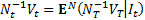
where  is
the information set (or filtration) generated by the underlying
processes and
is
the information set (or filtration) generated by the underlying
processes and  is
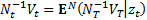
the relevant risk-neutral expectation operator. Usually, we will restrict
ourselves to Markovian models, in which case the above formula can also be
written as:
is
the relevant risk-neutral expectation operator. Usually, we will restrict
ourselves to Markovian models, in which case the above formula can also be
written as:
1.5 The observation underlying SALI is that if the
payout can be written as a function of the underlying Markov process then it
can be decomposed into the sum of a finite number of smooth subcomponents i.e.
as:
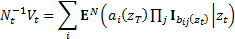
where  denotes
a (typically) low-dimensional underlying Markov process.
denotes
a (typically) low-dimensional underlying Markov process.
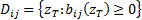
Here the  are
indicator functions, i.e.
are
indicator functions, i.e.  if
if  ,
,  otherwise.
The decomposition might use one smooth function between consecutive
discontinuities, or it might use several that are pasted together, e.g. cublic
spline functions.
otherwise.
The decomposition might use one smooth function between consecutive
discontinuities, or it might use several that are pasted together, e.g. cublic
spline functions.
1.6 The pricing problem can thus be re-expressed
as:
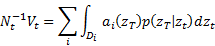
where  where
where
 .
.  can
in practice be truncated to be within some ‘envelope of support’ that includes
essentially all of the probability density applicable to the pricing problem.
For example, for a Weiner process, one might use an outer envelope spreading
out to, say, four standard deviations, since virtually none of the probability
density is outside this spread. However, care is needed in such a truncation if
the payoff function becomes sufficiently large sufficiently rapidly at the edge
of the distribution, see e.g. the Cost
of Capital pricing model.
can
in practice be truncated to be within some ‘envelope of support’ that includes
essentially all of the probability density applicable to the pricing problem.
For example, for a Weiner process, one might use an outer envelope spreading
out to, say, four standard deviations, since virtually none of the probability
density is outside this spread. However, care is needed in such a truncation if
the payoff function becomes sufficiently large sufficiently rapidly at the edge
of the distribution, see e.g. the Cost
of Capital pricing model.
NAVIGATION LINKS
Contents | Prev | Next