Deriving the Black-Scholes Option Pricing
Formulae using the limit of a suitably constructed lattice
[this page | pdf | references | back links]
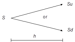
Suppose we knew for certain that between time  and
and
 the price of the
underlying could move from
the price of the
underlying could move from  to either
  or
to
or
to  , where
  (as in the diagram
below), that cash (or more precisely the appropriate risk-free asset) invested
over that period earns an interest rate (continuously compounded) of
(as in the diagram
below), that cash (or more precisely the appropriate risk-free asset) invested
over that period earns an interest rate (continuously compounded) of  and
that the underlying (here assumed to be an equity or an equity index) generates
income, i.e. dividend yield, (continuously compounded) of
and
that the underlying (here assumed to be an equity or an equity index) generates
income, i.e. dividend yield, (continuously compounded) of  .
.
Diagram illustrating single time-step binomial option
pricing
Suppose that we also have a derivative (or indeed any other
sort of security) which (at time ) is worth  if the share price has
moved to , and worth
if the share price has
moved to , and worth  if it has moved to .
Starting at at time , we
can (in the absence of transaction costs and in an arbitrage-free world)
construct a hedge portfolio at time that is guaranteed to
have the same value as the derivative at time whichever
outcome materialises. We do this by investing (at time )  in
in  units
of the underlying and investing
units
of the underlying and investing  in the risk-free
security, where and
in the risk-free
security, where and  satisfy
the following two simultaneous equations:
satisfy
the following two simultaneous equations:


Hence:

The value of the hedge portfolio and hence, by the principle
of no arbitrage, the value of the derivative at time can
thus be derived by the following backward equation:

We can rewrite this equation as follows, where 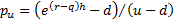 and
and 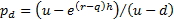 and hence
  .
.

Assuming that the two potential movements are chosen so that
 and
and  are both positive,
i.e. with
are both positive,
i.e. with 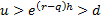 then and correspond to the
relevant risk neutral probabilities for the lattice element. Getting and to adhere to this
constraint is not normally difficult for an option like this since
then and correspond to the
relevant risk neutral probabilities for the lattice element. Getting and to adhere to this
constraint is not normally difficult for an option like this since  is the forward price
of the security and it would be an odd sort of binomial tree that did not
straddle the expected movement in the underlying.
is the forward price
of the security and it would be an odd sort of binomial tree that did not
straddle the expected movement in the underlying.
In the multi-period analogue, the price of the underlying is
assumed to be able to move in the first period either up or down by a factor  or
or  , and
in second and subsequent periods up or down by a further or from
where it had reached at the end of the preceding period. or can
in principle vary depending on the time period (e.g. might
be size
, and
in second and subsequent periods up or down by a further or from
where it had reached at the end of the preceding period. or can
in principle vary depending on the time period (e.g. might
be size  in time step
  ,
etc.) but it would then be usual to require the lattice to be recombining. In such a lattice an up movement in one time period followed by a down
movement in the next leaves the price of the underlying at the same value as a
down followed by an up. It would also be common, but again not essential (and
sometimes inappropriate), to have each time period of the same length,
,
etc.) but it would then be usual to require the lattice to be recombining. In such a lattice an up movement in one time period followed by a down
movement in the next leaves the price of the underlying at the same value as a
down followed by an up. It would also be common, but again not essential (and
sometimes inappropriate), to have each time period of the same length,  .
.
By repeated application of the backward equation referred to
above, we can derive the price  periods back, i.e. at
  , of a derivative with
an arbitrary payoff at time
, of a derivative with
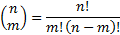
an arbitrary payoff at time  . If , , , , and are
the same for each period then:
. If , , , , and are
the same for each period then:
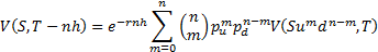
where:
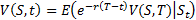
This can be re-expressed as an expectation under a risk-neutral probability distribution, i.e. in the following form, where  means the expected
value of
means the expected
value of  given the risk neutral
measure, conditional on being in state
given the risk neutral
measure, conditional on being in state  when the expectation
is carried out:
when the expectation
is carried out:
Suppose we have a European-style put option with strike
price  (assumed to be at a
node of the lattice) maturing at time and we want to
identify its price,
(assumed to be at a
node of the lattice) maturing at time and we want to
identify its price,  prior to maturity,
i.e. where
prior to maturity,
i.e. where  . Suppose also that and are
the same for each time period. The price of the option at maturity is given by
its payoff, i.e.
. Suppose also that and are
the same for each time period. The price of the option at maturity is given by
its payoff, i.e. 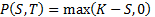 where
where 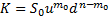 say for some
  (here
(here  is the price ruling at
time
is the price ruling at
time  used to construct the
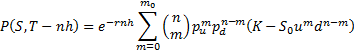
first node in the lattice). Applying the multi-period pricing formula set out
above, we find that the price of such an option at time
used to construct the
first node in the lattice). Applying the multi-period pricing formula set out
above, we find that the price of such an option at time  in such a framework is
as follows, where
in such a framework is
as follows, where  is the binomial
probability distribution function, i.e.
is the binomial
probability distribution function, i.e. 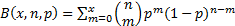 , bearing in mind that :

Suppose we define the volatility of the lattice to be
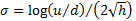 and suppose too that
this is constant, i.e. the same for each time period. Then if we allow to
tend to zero, keeping
and suppose too that
this is constant, i.e. the same for each time period. Then if we allow to
tend to zero, keeping  , , etc.
fixed, with
, , etc.
fixed, with  by, say, setting
  and
and  , we find that the
above formula and hence the price of the put option tends to:
, we find that the
above formula and hence the price of the put option tends to:

where
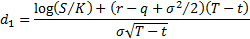
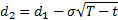
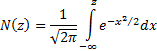
and  is the cumulative
Normal distribution function, i.e.
is the cumulative
Normal distribution function, i.e.
The corresponding formula (in the limit) for the price,  of a European call
option maturing at time with a strike price of
can be derived in an
equivalent manner as:
of a European call
option maturing at time with a strike price of
can be derived in an
equivalent manner as:

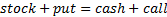
This formula can also be justified on the grounds that the
value of a combination of a European put option and a European call option with
the same strike price should satisfy so-called put-call parity,
if they are to satisfy the principle of no arbitrage, i.e. (after allowing for
dividends and interest):

Strictly speaking, these formulae for European put and call
options are the Garman-Kohlhagen formulae for
dividend bearing securities and only if is set to zero do they
become the original Black-Scholes option pricing formulae, although in
practice most people would actually refer to these formulae as the Black-Scholes
formulae, and call a world satisfying the assumptions underlying these formulae
as a ‘Black-Scholes’ world. The volatility used in their
derivation has a natural correspondence with the volatility that the share
price might be expected to exhibit in a Black-Scholes world.