Quantitative Return Forecasting
3. The spectrum and z-transform of
a time series
[this page | pdf | references | back links]
Return to Abstract and
Contents
Next page
3.1 An equivalent way of analysing a time series
is via its spectrum since we can transform a time series into a
frequency spectrum (and vice versa) using Fourier transforms. Take for example
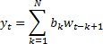
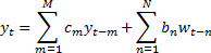
another sort of prototypical time series model, i.e. the moving average or
MA model. This assumes that the output depends purely on an input series
(without autoregressive components), i.e.:
3.2 There are three equivalent characterisations
of a  model:
(a)
In the time domain - i.e. directly via the  .
.
(b)
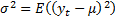
In the form of autocorrelations, i.e. 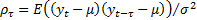 (where
 means
the expected value of
means
the expected value of  and
and  and
and
 .
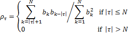
If the input to the system is a stochastic process with input values at
different times being uncorrelated (i.e.
.
If the input to the system is a stochastic process with input values at
different times being uncorrelated (i.e.  for
for
 )
then the autocorrelation coefficients become:
)
then the autocorrelation coefficients become:
(c)
In the frequency domain. If the input to a model is
an impulse then the spectrum of the output (i.e. the result of applying the
discrete Fourier transform to the time series) is given by:

3.3 It is possible to show that an AR model
of the form described earlier has a power spectrum of the following form:  .
The obvious next step in complexity is to have both AR and MA components in the
same model, e.g. an
.
The obvious next step in complexity is to have both AR and MA components in the
same model, e.g. an  model,
of the following form:
model,
of the following form:
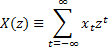
3.4 The output of an  model is
most easily understood in terms of the z-transform, which generalises
the discrete Fourier transform to the complex plane, i.e.:
model is
most easily understood in terms of the z-transform, which generalises
the discrete Fourier transform to the complex plane, i.e.:
3.5 On the unit circle in the complex plane the z-transform
reduces to the discrete Fourier transform. Off the unit circle, it measures the
rate of divergence or convergence of a series. Convolution of two series in the
time domain corresponds to the multiplication of their z-transforms.
Therefore the z-transform of the output of an model
is:
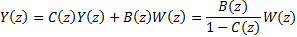
3.6 This has the form of an input z-transform
 multiplied
by a transfer function
multiplied
by a transfer function 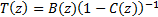 unrelated
to the input. The transfer function is zero at the zeros of the term,
i.e. where
unrelated
to the input. The transfer function is zero at the zeros of the term,
i.e. where  ,
and diverges to infinity, i.e. has poles (in a complex number sense), where
,
and diverges to infinity, i.e. has poles (in a complex number sense), where  ,
unless these are cancelled by zeros in the numerator. The number of poles and
zeros in this equation determines the number of degrees of freedom in
the model. Since only a ratio appears there is no unique model
for any given system. In extreme cases, a finite-order
,
unless these are cancelled by zeros in the numerator. The number of poles and
zeros in this equation determines the number of degrees of freedom in
the model. Since only a ratio appears there is no unique model
for any given system. In extreme cases, a finite-order  model
can always be expressed by an infinite-order model,
and vice versa.
model
can always be expressed by an infinite-order model,
and vice versa.
3.7 There is no fundamental reason to expect an
arbitrary model to be able to be described in an form.
However, if we believe that a system is linear in nature then it is reasonable
to attempt to approximate its true transfer function by a ratio of polynomials,
i.e. as an model. This is a problem in
function approximation. It can be shown that a suitable sequence of ratios of
polynomials (called Padé approximants) converges faster than a power series
for an arbitrary function. But this still leaves unresolved the question of
what the order of the model should be, i.e. what values of  and
and  to
adopt. This is in part linked to how best to approximate the z-transform.
There are several heuristic algorithms for finding the ‘right’ order, for
example the Akaike Information Criterion, see e.g. Billah,
Hyndman and Koehler (2003). These heuristic approaches usually rely very
heavily on the model being linear and can also be sensitive to the assumptions
adopted for the error terms.
to
adopt. This is in part linked to how best to approximate the z-transform.
There are several heuristic algorithms for finding the ‘right’ order, for
example the Akaike Information Criterion, see e.g. Billah,
Hyndman and Koehler (2003). These heuristic approaches usually rely very
heavily on the model being linear and can also be sensitive to the assumptions
adopted for the error terms.
3.8 This point is also related to the distinction
between in-sample and out-of-sample analysis. By in-sample we
mean an analysis carried out on a particular data set not worrying about the
fact that later observations would not have been know about at earlier times in
the analysis. If, as will always be the case in practice, the data series is
finite then incorporating sufficient parameters in the model will always enable
us to fit the data exactly (in much the same way that a sufficiently high order
polynomial can always be made to fit exactly a fixed number of points on a
curve).
3.9 What normally happens is that the researcher
will choose one period of time to estimate the parameters characterising the
model and will then test the model out-of-sample using data for a
subsequent (but still historic) time period. Sometimes the parameters will be
fixed at the end of the in-sample period.
3.10 Alternatively, if we have some a priori
knowledge about the nature of the linear relationship then our best estimate at
any point in time will be updated as more knowledge becomes available in a
Bayesian fashion. Updating estimates of the linear parameters in this manner is
usually called applying a Kalman filter to the process, a technique that
is also used in general insurance claims reserving.
3.11 In derivative pricing there is a similar need
to avoid look-forward bias, and this is achieved via the use of so called adapted
series, i.e. random series where you do not know what future impact the
randomness being assumed will have until you reach the relevant point in time
when the randomness arises.
3.12 However, it is worth bearing in mind that even
rigorous policing of in-sample and out-of-sample analysis does not avoid an
implicit element of ‘look-forward-ness’ when carrying out back tests of how a
particular quantitative return forecasting might perform in the future. This is
because the forecasters can be thought of as having a range of possible models
from which they might choose. They are unlikely to present results where
out-of-sample behaviour is not as desired. Given a sufficiently large number of
possible model types, it is always be possible to find one consistent with an
in-sample analysis that also looks good in a subsequent out-of-sample analysis.
By the time we do the analysis we actually know what happened in both periods.
NAVIGATION LINKS
Contents | Prev | Next