Relative Value-at-Risk (Relative VaR)
[this page | pdf | back links]
Suppose we want to derive the (relative) portfolio
Value-at-Risk (relative VaR) when returns  on
the
on
the  exposures
are jointly Gaussian, assuming that the corresponding portfolio weights are
exposures
are jointly Gaussian, assuming that the corresponding portfolio weights are  and
corresponding benchmark weights are
and
corresponding benchmark weights are  .
.
By jointly Gaussian we mean that the vector of returns  is
distributed as a multivariate normal distribution
is
distributed as a multivariate normal distribution  ,
where
,
where  is
a vector of mean returns and
is
a vector of mean returns and  is
a covariance matrix.
is
a covariance matrix.
A property of any -dimensional Gaussian, i.e.
multivariate Normal, distribution that can be derived relatively simply from
the probability density function of such a distribution is that if  and
if we have a constant vector
and
if we have a constant vector  then
then
 is
univariate Normal
is
univariate Normal  for
some
for
some  and
and
 .
Specifically:
.
Specifically:

where the  are
the elements of the covariance matrix .
are
the elements of the covariance matrix .
By relative return we mean the return on the portfolio
relative to the return on the benchmark. For any given time period the return
on the portfolio is the weight the portfolio ascribes to the exposure times the
return on that exposure, i.e. is  ,
where
,
where  is
a vector with components
is
a vector with components  .
Likewise the return on the benchmark is is
.
Likewise the return on the benchmark is is 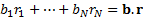 ,
where
,
where  is
a vector with components
is
a vector with components  .
So the relative return* is
.
So the relative return* is  .
Hence the relative return is distributed as a univariate Normal distribution
with
.
Hence the relative return is distributed as a univariate Normal distribution
with  and
and
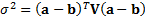 .
The relative VaR with confidence level
.
The relative VaR with confidence level  is
then
is
then 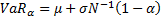 with
these and
with
these and  , where
  is
the inverse Normal function.
is
the inverse Normal function.
* N.B. there is an assumption here that the returns over the
relevant time interval are small, otherwise there is an issue about whether to
use arithmetic relative or geometric relatives etc., see e.g. Relative Return
Computations).