Enterprise Risk Management Formula Book
5. Statistical Methods
[this page | pdf | back links]
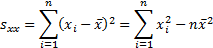
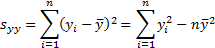
5.1 Sample moments
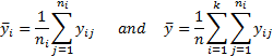
A random sample of  observations
  has (equally
weighted) sample moments as follows:
has (equally
weighted) sample moments as follows:
‘Population’ moments (e.g. population variance,
population skewness,
population excess
kurtosis) are calculated as if the distribution from which the data was
being drawn was discrete and the probabilities of occurrence exactly matched
the observed frequency of occurrence.
The least squares estimator for parameters of a distribution
are the values of the parameters that minimise the square of the residuals, so
the least squares estimator for the mean,  , is the value
that minimises
, is the value
that minimises 
Non-equally weighted moments give different weights to
different observations (the weights not dependent on the ordering of the
observations), e.g. the sample non-equally weighted mean (using
weights  ) is:
) is:

5.2 Parametric inference (with an underlying
following the normal distribution)
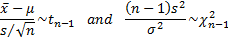
One sample:
For a single (equally weighted) sample of size ,
, where  then the
following statistics are distributed according to the Student’s t
distribution and the chi-squared distribution:
then the
following statistics are distributed according to the Student’s t
distribution and the chi-squared distribution:
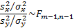
Two samples:
For two independent samples of sizes  and
,
and
,  and
and  , where
  and
and  then the
following statistic is
distributed according to the F distribution:
then the
following statistic is
distributed according to the F distribution:
If  then:
then:

where 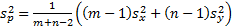 is the pooled
sample variance.
is the pooled
sample variance.
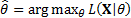
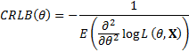
5.3 Maximum likelihood estimators
If  is the maximum likelihood estimator
of a parameter
is the maximum likelihood estimator
of a parameter  based on a
sample
based on a
sample  then
then
where  is the
likelihood for the sample, i.e.
is the
likelihood for the sample, i.e.  and hence
is
asymptotically normally distributed with mean and
variance equal to the Cramér-Rao lower bound
Likelihood ratio test:
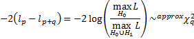
where  is the
maximum log-likelihood for the model under
is the
maximum log-likelihood for the model under  (with
(with  free
parameters) and
free
parameters) and 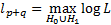 is the
maximum log-likelihood for the model under
is the
maximum log-likelihood for the model under  (with
(with  free
parameters). Non-equally weighted estimators can be identified by weighting the
free
parameters). Non-equally weighted estimators can be identified by weighting the
 terms
appropriately.
terms
appropriately.
5.4 Method-of-moments estimators
Method of moments estimators are the parameter values
(for the parameters
specifying a given distributional family) that result in replication of the
first moments of
the observed data. For the normal distribution these involve 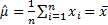 and either
 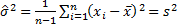 (the sample
variance, if a small sample size adjustment is included) or
(the sample
variance, if a small sample size adjustment is included) or 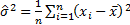 (the
‘population’ variance, if the small sample size adjustment is ignored and we
select the estimators to fit
(the
‘population’ variance, if the small sample size adjustment is ignored and we
select the estimators to fit  and
and  . In the generalised
method of moments approach we select parameters that ‘best’ fit the
selected moments (given some criterion for ‘best’), rather than selecting
parameters that perfectly fit the selected moments.
. In the generalised
method of moments approach we select parameters that ‘best’ fit the
selected moments (given some criterion for ‘best’), rather than selecting
parameters that perfectly fit the selected moments.
5.5 Goodness of fit
Goodness of fit describes how well a statistical model fits
a set of observations. Examples include the following, where  is the
  ’th
order statistic,
’th
order statistic,  is the
supremum (i.e. largest value) of the set
is the
supremum (i.e. largest value) of the set  ,
,  is
the cumulative distribution function of the distribution we are fitting and
is
the cumulative distribution function of the distribution we are fitting and  is the
empirical distribution function:
is the
empirical distribution function:
(a) Kolmogorov-Smirnov
test: 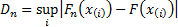 . Under the
null hypothesis (that the sample comes from the hypothesized distribution), as
. Under the
null hypothesis (that the sample comes from the hypothesized distribution), as  then
then
 tends to a
limiting distribution (the Kolmogorov distribution).
tends to a
limiting distribution (the Kolmogorov distribution).
(b) Cramér-von-Mises test: 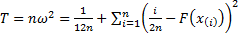
(c) Anderson-Darling test:
 where
where 
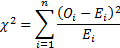
If data is bucketed into ranges then we may also use
(Pearson’s) chi-squared goodness of fit test using the following test
statistic, where is the sample
size and  is the
observed count,
is the
observed count, 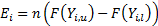 is the
expected count and
is the
expected count and  and
and  are the lower
and upper limits for the ’th bin. The test
statistic follows approximately a chi-squared distribution with
are the lower
and upper limits for the ’th bin. The test
statistic follows approximately a chi-squared distribution with  degrees
of freedom, i.e.
degrees
of freedom, i.e.  where
where  is
the number of non-empty cells and
is
the number of non-empty cells and  is the number
of estimated parameters plus 1:
is the number
of estimated parameters plus 1:
We may also test whether the skew or kurtosis or the two
combined (the Jarque-Bera test) appear materially different from what would be
implied by the relevant distributional family. If the null hypothesis is that
the data comes from a normal distribution then, for large ,
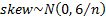 ,
, 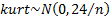 and
and 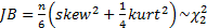 .
.
The Akaike
Information Criterion (AIC) (and other similar ways of choosing between
different types of model that trade-off goodness of fit with model complexity,
such as the Bayes Information Criterion, BIC) involves selecting the
model with the highest information criterion of the form 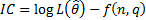 where there
are
where there
are  unknown
parameters and we are using a data series of length for
fitting purposes. For the AIC
unknown
parameters and we are using a data series of length for
fitting purposes. For the AIC  and for the
BIC
and for the
BIC 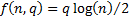 .
.
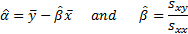
5.6 Linear regression
In the univariate case suppose 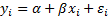 where
where  ,
,  then
(equally weighted) estimates of
then
(equally weighted) estimates of  and
and  are:
are:
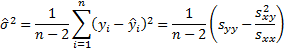
where
Also

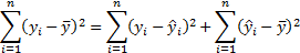
The individual expected responses are  and satisfy
the following ‘sum of squares’ relationship:
and satisfy
the following ‘sum of squares’ relationship:
The variance of the predicted mean response is:
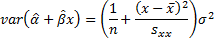
The variance of a predicted individual response is the
variance of the predicted mean response plus an additional  .
.
For generalised least squares, if we have different
series each with observations
we are fitting 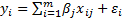 then the
vector of least squares estimators,
then the
vector of least squares estimators, 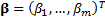 is given by
 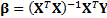 where
where  is a
is a  matrix
with elements
matrix
with elements  and
and  is an dimensional
vector with elements
is an dimensional
vector with elements  .
.
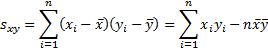
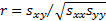
5.7 Correlations
The observed (sample) correlation coefficient
(i.e. Pearson correlation coefficient) between two series of equal
lengths indexed in the same manner  and
and  is (where
  ,
,  and
and  are as given
in the section on linear regression):
are as given
in the section on linear regression):
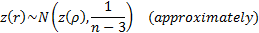
If the underlying correlation coefficient,  ,
is zero and the data comes from a bivariate normal distribution then:
,
is zero and the data comes from a bivariate normal distribution then:

For arbitrary ( )
the Fisher z transform
is
)
the Fisher z transform
is  where:
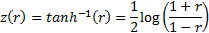
If the data comes from a bivariate normal distribution then is
distributed approximately as follows:
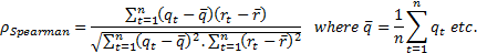
Two non-parametric measures of correlation are:
-
Spearman’s
rank correlation coefficient, where  and
and  are the ranks
within
are the ranks
within  and
and  of
of
 and
and  respectively:
-
Kendall’s
tau, where computation is taken over all  and
and
 with
with  and
(for the moment ignoring ties) a concordant pair is a case where
and
(for the moment ignoring ties) a concordant pair is a case where  and a
discordant pair is a case where
and a
discordant pair is a case where  :
:
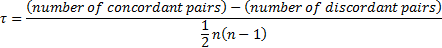
There are various possible ways of handling ties in these
two non-parametric measures of correlation (ties should not in practice arise
if the random variables really are continuous).
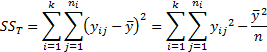
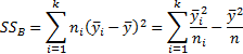
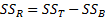
5.8 Analysis of variance
Given a single factor normal model

where  with
with  .
.
Variance estimate:

Under the null hypothesis given above
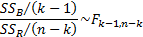
where:
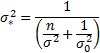
5.9 Bayesian priors and posteriors
Posterior and prior distributions are related as follows:

i.e.
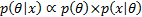
For example, if is a random
sample of size from a  where is known and
the prior distribution for
where is known and
the prior distribution for  is
is  then the
posterior distribution for is:
then the
posterior distribution for is:

where  is
‘credibility weighted’ as follows:
is
‘credibility weighted’ as follows:

and
NAVIGATION LINKS
Contents | Prev | Next