Calculating TVaR if a distribution has a
quantile-quantile form (versus the normal distribution) that is a cubic
polynomial
[this page | pdf | references | back links]
A method that some practitioners use to estimate risk
measures such as Value-at-Risk
(VaR) and Tail
Value-at-Risk (TVaR) for fat-tailed distributions is make use of the
Cornish-Fisher asymptotic expansion, see derivation of the
Cornish-Fisher expansion or MnCornishFisher4.
This is a methodology for predicting the shape of a (univariate) distributional
form merely from the moments of the distribution, most commonly merely its
mean, standard deviation, skew and (excess) kurtosis.
However, Kemp (2009) notes
that the Cornish-Fisher approach has some undesirable features including not
necessarily giving appropriate weight to different parts of the distributional
form. In effect it can result in estimation of outlying quantiles of the
distribution more from the distributional shape in the centre of the
distribution than from its shape in its tails, which is counterintuitive and
liable to error. Kemp proposes a more empirical approach in which the
distributional form and hence the risk measure is derived from a curve that is
directly fitted to the shape of the quantile-quantile plot, possibly giving
greater weight to observations in this curve fitting process to regions of the
distribution that the user is most interested in analysing. His suggested curve
form to use for this purpose is a cubic, since the fourth moment Cornish-Fisher
approach is in effect also characterised by a cubic quantile-quantile plot but
not necessarily one giving the most suitable weights to different parts of the
distributional form.
As noted in Kemp (2009)
such an approach also simplifies computation of TVaR risk measures.
Suppose the quantile-quantile plot (versus the corresponding
standardised normal distribution) takes a cubic form, i.e. is of the form  . Not
all choices of
. Not
all choices of  correspond
to a valid probability distribution. Real vaued probability distributions must
have monotonically non-decreasing cumulative distribution functions, which in
this instance means that
correspond
to a valid probability distribution. Real vaued probability distributions must
have monotonically non-decreasing cumulative distribution functions, which in
this instance means that  needs
to be non-decreasing for all
needs
to be non-decreasing for all  ,
which requires
,
which requires  and
and 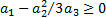 .
.
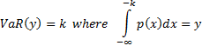
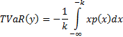
If the cubic does correspond to a valid probability
distribution then the VaR and TVaR of the distribution, for a given confidence
level  , are
defined as follows, where
, are
defined as follows, where  is
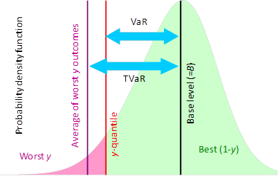
the distribution’s probability density function (assuming that we adopt the
same definition for TVaR as is used in the illustrative chart below and
suitably rebase the -axis,
i.e. here set
is
the distribution’s probability density function (assuming that we adopt the
same definition for TVaR as is used in the illustrative chart below and
suitably rebase the -axis,
i.e. here set  ):
):
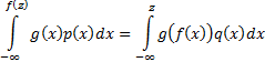
At first sight these integrals look quite complicated to
evaluate, since they appear to require us to derive .
However we note that in this instance the following relationship applies for an
arbitrary  satisfying
appropriate regularity conditions, where
satisfying
appropriate regularity conditions, where  is
the probability density function of the corresponding normal distribution
(with, say, mean
is
the probability density function of the corresponding normal distribution
(with, say, mean  and
standard deviation
and
standard deviation  ) and
) and
 is
the standard inverse normal
function:
is
the standard inverse normal
function:
VaR corresponds to the case where  ,
i.e. can be evaluated, as we might expect as:
,
i.e. can be evaluated, as we might expect as:

TVaR corresponds to the case where  ,
i.e.
,
i.e.  and
thus can be derived analytically (as a function of
and
thus can be derived analytically (as a function of  , and
deeming to
be ‘analytic’) using methodologies set out in integrating
piecewise polynomials against a Gaussian probability density function.
, and
deeming to
be ‘analytic’) using methodologies set out in integrating
piecewise polynomials against a Gaussian probability density function.