Random Matrix Theory
[this page | pdf | references | back links]
Tools
References
The risks expressed by a portfolio of assets or liabilities
depend heavily on how these assets and liabilities might ‘co-move’, i.e. move
in tandem. One way of analysing these co-movement characteristics is to
consider the covariances between the price movements of (or more precisely, the
log returns on) different assets and liabilities.
Most usually, investigators encapsulate this information
within a single structure, the covariance matrix, often estimating this matrix
empirically, using past observed covariances between the different assets and
liabilities.
But how do we tell how ‘reliable’ is this estimation
process? Suppose we have  time periods that we can
use to estimate empirically the characteristics of the covariance matrix and
time periods that we can
use to estimate empirically the characteristics of the covariance matrix and  assets
or liabilities (i.e. ‘instruments’). The correlation matrix contains
assets
or liabilities (i.e. ‘instruments’). The correlation matrix contains  distinct
entries. If is large relative to (which it
usually is in the risk management context) then we should expect the empirical
determination of the covariance matrix to be ‘noisy’, i.e. for it to have a
material element of randomness derived from measurement ‘noise’. It should
therefore be used with caution. Such matrices can be characterised by their
eigenvectors and eigenvalues, and it is the smallest (and hence apparently
least relevant) of these that are most sensitive to this noise. But these are
precisely the ones that determine, in Markowitz theory, the precise structure
of optimal portfolios, see Laloux et
al. (1999).
distinct
entries. If is large relative to (which it
usually is in the risk management context) then we should expect the empirical
determination of the covariance matrix to be ‘noisy’, i.e. for it to have a
material element of randomness derived from measurement ‘noise’. It should
therefore be used with caution. Such matrices can be characterised by their
eigenvectors and eigenvalues, and it is the smallest (and hence apparently
least relevant) of these that are most sensitive to this noise. But these are
precisely the ones that determine, in Markowitz theory, the precise structure
of optimal portfolios, see Laloux et
al. (1999).
It is thus desirable to devise ways of distinguishing
between ‘signal’ and ‘noise’, i.e. to distinguish between those eigenvalues and
eigenvectors of the covariance matrix that appear to correspond to real
characteristics exhibited by these assets and liabilities and those that are
mere artefacts of this noise.
One way of doing this is to use random matrix theory. This
theory has a long history in physics since Eugene Wigner and Freeman Dyson in
the 1950s. It aims to characterise the statistical properties of the
eigenvalues and eigenvectors of a given statistical ‘ensemble’ (i.e. the set of
random matrices exhibiting pre-chosen symmetries or other sorts of
constraints). Amongst other things, we might be interested in the average
density of eigenvalues and in the distribution of spacing between consecutively
ordered eigenvalues etc.
For example, we might compare the properties of an empirical
covariance matrix  with a ‘null hypothesis’
that the assets were, in fact, uncorrelated. Deviations from this null
hypothesis that were sufficiently unlikely might then suggest the presence of
true information.
with a ‘null hypothesis’
that the assets were, in fact, uncorrelated. Deviations from this null
hypothesis that were sufficiently unlikely might then suggest the presence of
true information.
In the limit of very large matrices (i.e.  ) this density
is analytically tractable and is as follows, for covariance matrices derived
from (independent) series that have a common standard deviation,
) this density
is analytically tractable and is as follows, for covariance matrices derived
from (independent) series that have a common standard deviation,  .
Correlation matrices derived from the above null hypothesis have this property,
as they correspond to covariance matrices where each series has a standard
deviation in isolation of
.
Correlation matrices derived from the above null hypothesis have this property,
as they correspond to covariance matrices where each series has a standard
deviation in isolation of  .
.
The density, for a given  ,
is
,
is  where:
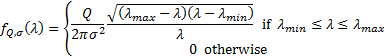
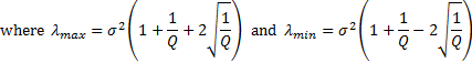
In the limiting case where is large
this has some features that get smoothed out in practice for less extreme
values of , in particular the
existence of a hard upper and (if  ) lower limit above and
below which the density falls to zero.
) lower limit above and
below which the density falls to zero.
We may therefore adopt the following prescription for
‘denoising’ an empirically observed correlation matrix, if we can assume that
the ‘null’ hypothesis is that the instruments are independent (an assumption
that would be inappropriate if, say, we should ‘expect’ two instruments to be
correlated, e.g. the two might be listings of the same underlying asset on two
different stock exchanges, or two bonds of similar terms issued by the same
issuer), see Scherer
(2007):
(a) Work out the
empirically observed correlation matrix (which by construction has standardised
the return series so that ).
(b) Identify the largest
eigenvalue and corresponding eigenvector of this matrix.
(c) If the
eigenvalue is sufficiently large, e.g. materially larger than the cut-off
derived from the above (or some more accurate determination of the null
hypothesis density applicable to the finite case),
then deem the eigenvalue to represent true information rather than noise and
move on to step (d), otherwise stop.
(d) Record the eigenvalue
and corresponding eigenvector. Determine the contribution to each instrument’s
return series from this eigenvector. Strip out these contributions from each
individual instrument return series, calculate a new correlation matrix for
these adjusted return series and loop back to (b).
The reason we in theory need to adjust each instrument
return series in step (d) is that otherwise the ‘residual’ return series can no
longer be assumed to have a common , so we can no longer
directly use a formula akin to that above to identify further eigenvectors that
appear to encapsulate true information rather than noise. However, if we ignore
this nicety (i.e. we adopt the null hypothesis that all residual return series,
after stripping out ‘significant eigenvectors’ are independent identically
distributed Gaussian random series with equal standard deviations) then the
computation of the cut-offs simplifies materially. This is because:
i.
The trace of a symmetric matrix (i.e. the sum of the leading diagonal
elements) is the same as the sum of its eigenvectors (and is therefore
invariant relative to a change in basis for the relevant vector space).
ii.
So, removing the leading eigenvector as above merely involves removing
the leading row and column, if the basis used involves the eigenvectors.
iii.
The variance of the residual series under this null hypothesis is
therefore merely the sum of the eigenvalues not yet eliminated iteratively.
iv.
Hence, we can calculate the cutoff  for
the
for
the  ’th eigenvalue (
 as
follows, where
as
follows, where  is
the magnitude of the
is
the magnitude of the  ’th eigenvalue (
 :
:
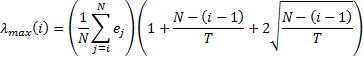
Using this prescription, we would exclude any eigenvalues
and corresponding eigenvectors beyond the first one for which the eigenvalue is
not noticeably above this cutoff. The Nematrian website function MnEigenvalueSpreadsForRandomMatrices
calculates these .
More precise tests of significance could be identified by simulating spreads of
results for random matrices.
Edelman and
Rao (2005) describe how in many cases it is possible to calculate
eigenvalue densities for a wide range of transformations of random matrices,
including both deterministic and stochastic transformations. They express the
view that the usefulness of random matrix theory will through time follow that
of numerical analysis more generally, i.e. most disciplines in science and
engineering will in due course find random matrix theory a valuable tool. Its
history started in the physics of heavy atoms and multivariate statistics. It
has already found its way into wireless communications and combinatorial
mathematics and as seen above is potentially also becoming increasingly used in
the field of financial analysis and risk management.
NAVIGATION LINKS
Contents | Next