Extreme Value Theory
3. Main Block maxima results and the
Fisher-Tippett, Gnedenko theorem
[this page | pdf | references | back links]
Return
to Abstract and Contents
Next
page
As noted in the Introduction,
‘block maxima’ results are the more traditional variant of EVT but are also
less useful for risk management purposes as they are less directly relevant to
the task of, say, estimating VaR’s at extreme threshold levels. However, it is
conventional to discuss these first, so we also develop EVT in this manner.
Suppose we are interested in statistics applicable to a set
of portfolio losses measured over time. We assume that these losses are random
variables. These losses will be a series  ,
say. We will first assume that the losses are independent and identically
distributed (‘i.i.d’) but later we will relax this assumption. We will also
assume that the
,
say. We will first assume that the losses are independent and identically
distributed (‘i.i.d’) but later we will relax this assumption. We will also
assume that the  are
continuous random variables.
are
continuous random variables.
The role of the generalised extreme value (GEV) distribution
in the theory of extremes
Is analogous to the role the normal distribution plays
within the Central Limit Theorem (CLT). With the CLT we have to normalise
the data for a limiting distribution to appear. Specifically, if  are
iid with a finite variance and if we write
are
iid with a finite variance and if we write  then
the CLT indicates that appropriately normalised sums,
then
the CLT indicates that appropriately normalised sums,  converge
in distribution to the standard normal, i.e. the
converge
in distribution to the standard normal, i.e. the  ,
distribution as
,
distribution as  tends to infinity. By
‘normalise’ we here mean a sequence of normalising constants not dependent on
any particular but
dependent merely on and on the parameters
characterising the distribution from which they are all drawn. For the CLT the
normalising constants
tends to infinity. By
‘normalise’ we here mean a sequence of normalising constants not dependent on
any particular but
dependent merely on and on the parameters
characterising the distribution from which they are all drawn. For the CLT the
normalising constants  and
and
 are
defined by
are
defined by  and
and
 .
In mathematical notation we have:
.
In mathematical notation we have:
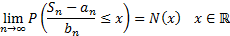
where  is the cumulative
distribution function of the unit normal distribution.
is the cumulative
distribution function of the unit normal distribution.
Block maxima results focus on suitably normalised maxima of
discrete sets of .
So, suppose each block consists of elements (so the  ’th block
involves elements numbered
’th block
involves elements numbered  to
to  (if the first entry in the
series is numbered entry 1). We calculate
(if the first entry in the
series is numbered entry 1). We calculate  and
we are interested in the distributional form of
and
we are interested in the distributional form of  (appropriately
normalised) as
(appropriately
normalised) as  . If the available observed
data involves
. If the available observed
data involves  such blocks, i.e. is of
length
such blocks, i.e. is of
length  , say, then we will have
only different (independent)
values of .
In some loose sense only ‘one’ data point from each block drives and
any information implicit in the remainder is thrown away by focusing merely on
these maxima (although of course all in some underlying sense influence ).
Thus the approach appears likely to make relatively inefficient use of the
available data when applied to real life data series, if is
large.
, say, then we will have
only different (independent)
values of .
In some loose sense only ‘one’ data point from each block drives and
any information implicit in the remainder is thrown away by focusing merely on
these maxima (although of course all in some underlying sense influence ).
Thus the approach appears likely to make relatively inefficient use of the
available data when applied to real life data series, if is
large.
Suppose the cumulative distribution function of each is
 ,
then because they are i.i.d. we will have
,
then because they are i.i.d. we will have 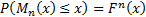
The main block maxima EVT result is then as follows:
(1) Suppose
that there are real sequences of numbers  and
and
 ,
where
,
where  for
all such that:
for
all such that:
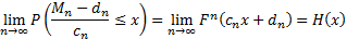
for some
non-degenerate  (by
non-degenerate we mean that the limiting distribution is not concentrated onto
a single point).
(by
non-degenerate we mean that the limiting distribution is not concentrated onto
a single point).
(2)  is then
said to be in the maximum domain of attraction of
is then
said to be in the maximum domain of attraction of  ,
written
,
written  .
.
(3) The
Fisher-Tippett, Gnedenko Theorem states that if for
some non-degenerate distribution function then
(when
appropriately standardised) must represent a generalised extreme value (GEV) distribution,  ,
for some value of
,
for some value of  . Such a distribution has a
distribution function:
. Such a distribution has a
distribution function:
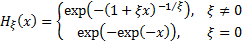
where  .
.
A (non-standardised) three-parameter family is obtained by
defining 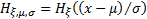 for
a location parameter
for
a location parameter  and
a scale parameter
and
a scale parameter  . It is always possible to
choose and
so
that the resulting distribution takes the standard form. Some commentators
replace by
. It is always possible to
choose and
so
that the resulting distribution takes the standard form. Some commentators
replace by  to
make the link with Pareto distributions clearer (see threshold exceedance
results). If
to
make the link with Pareto distributions clearer (see threshold exceedance
results). If  is
positive then it is known as the tail index, for reasons set out below.
is
positive then it is known as the tail index, for reasons set out below.
The GEV is ‘generalised’ in the sense that it subsumes three
types of distribution which are known by other names, i.e.:
The Weibull distribution is a short-tailed distribution with
a so-called finite right endpoint,  .
The Gumbel and Fréchet
distributions have infinite right end points, but the decay in the tail of the Fréchet
distribution is much slower than for the Gumbel distribution.
.
The Gumbel and Fréchet
distributions have infinite right end points, but the decay in the tail of the Fréchet
distribution is much slower than for the Gumbel distribution.
NAVIGATION LINKS
Contents | Prev | Next