Extreme Events – Specimen Question
A.5.1(a) – Answer/Hints
[this page | pdf | references | back links]
Return
to Question
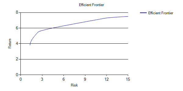
Q. Plot the efficient
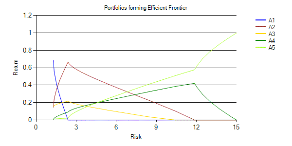
frontier and the asset mixes making up the points along the efficient frontier,
assuming that risk-free is to be equated with zero volatility of return and
that no non-negative holdings are allowed for any asset category.
The efficient frontier can be found using standard
constrained quadratic optimisation techniques, constrained
quadratic optimisation techniques and then plotting the results.
This can be done using the Solver add-in that comes as
standard with Microsoft Excel, but rather simpler (in our opinion) is to make
use of the Nematrian online toolkit or an equivalent. The Nematrian toolkit
provides three different tools, each one of which can be used to solve this
particular problem:
(a) The asset mix
(and corresponding risk and expected return) corresponding to a single
point along the efficient frontier (i.e. for a specific  , i.e.
risk-reward trade-off parameter) can be found interactively using Nematrian’s Example
Quadratic Portfolio Optimiser page.
(b) In this case we
want to plot the efficient frontier, i.e. we want the risk and expected returns
for a range of points along the efficient frontier (and we also want to plot
the corresponding asset mixes). We could run (a) for several different
efficient frontiers, but this would be quite laborious. Simpler than (a)
(particularly if you are likely to carry out several similar exercises) may be
to call the corresponding Nematrian MnConstrainedQuadraticPortfolioOptimiser
web service function many times using VBA.
(c) Perhaps
best in this instance is to piggy-back off of the Nematrian website’s SmartChart facility
and to use the (standard) Nematrian web function plotting equivalents to (b),
i.e. MnPlotQuadraticEfficientFrontier
and MnPlotQuadraticEfficientPortfolios
respectively. The web function itself returns a string corresponding to the
SmartCode of a suitable Smart Chart. The interactive variant returns an entire
(temporary) Nematrian SmartChart (which incorporates this SmartCode).
Even simpler, if it exists, is to use a previously
established spreadsheet that embeds the relevant Nematrian web functions. For
this particular purpose one does exist and can be found here.
Other spreadsheets that simultaneously illustrate a selection of related
Nematrian web functions can be found here.
Permanent SmartCharts corresponding to (c) are shown below.
To equate risk free with zero volatility the minimum risk portfolio should be
input as {0,0,0,0,0}. To bar non-negative holdings, place a lower limit of zero
on each holding, i.e. the Lower Bounds should be input as {0,0,0,0,0}. Asset
weights must add to unity, which can be achieved by suitable choice of
Constraint Matrix, Constraint Limits and Constraint Types. A full symmetric
correlation matrix needs to be input into Forecast Correlations, i.e. here:
|
|
A1
|
A2
|
A3
|
A4
|
A5
|
|
A1
|
1
|
0.4
|
-0.6
|
0.0
|
-0.4
|
|
A2
|
0.4
|
1
|
-0.5
|
-0.4
|
-0.4
|
|
A3
|
-0.6
|
-0.5
|
1
|
0.2
|
0.6
|
|
A4
|
0.0
|
-0.4
|
0.2
|
1
|
0.3
|
|
A5
|
-0.4
|
-0.4
|
0.6
|
0.3
|
1
|
Some playing around with the input lambda values may be
needed to get a set that span the entire range of efficient portfolios. For the
charts below we have used the following input values of lambda:
|
0.1
|
|
1
|
|
2
|
|
3
|
|
4
5
|
|
7
|
|
10
|
|
12
|
|
14
|
|
16
|
|
18
|
|
20
|
|
25
|
|
30
|
|
35
|
|
40
|
|
45
|
|
50
|
|
60
|
|
70
|
|
80
|
|
90
|
|
100
|
|
125
|
|
150
|
|
175
|
|
200
|
|
300
|
|
400
|
|
500
|
|
600
|
|
700
|
|
900
|
Efficient frontier:

Portfolios forming the efficient frontier

NAVIGATION LINKS
Contents | Prev | Next | Question