Extreme Events – Specimen Question
A.2.2(b) – Answer/Hints
[this page | pdf | references | back links]
Return
to Question
Q. Using a first order
autoregressive model, de-smooth the observed returns for Index B to derive a
return series that you think may provide a better measure of the underlying
behaviour of the relevant asset category.
The approach for de-smoothing (or ‘de-correlating’) such
returns suggested in the book Extreme Events involves
assuming that there is some underlying ‘true’ return series,  , and that
the observed series,
, and that
the observed series,  , derives
from it via a first order autoregressive model,
, derives
from it via a first order autoregressive model,  . We will
assume that the autoregressive model actually applies to the logged returns,
which are given in ExtremeEventsQuestionsAndAnswers2_1a.
. We will
assume that the autoregressive model actually applies to the logged returns,
which are given in ExtremeEventsQuestionsAndAnswers2_1a.
If we assume that the corresponding are
independent, identically distributed (normal) random variables with standard
deviation  (and mean
0 given that we have standardised the data) then the (expected) variance of the
series
(and mean
0 given that we have standardised the data) then the (expected) variance of the
series  , will be
  and the
(expected) covariance of the series
and the
(expected) covariance of the series  with the
series
with the
series  will be
  .
.
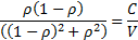
One way of proceeding would be to estimate  as
the solution to the equation:
as
the solution to the equation:
More precisely, since the above does not differentiate
between and  we
would probably choose the closest
to zero (and, ideally, we would expect it to be positive and smaller than 0.5,
which also requires
we
would probably choose the closest
to zero (and, ideally, we would expect it to be positive and smaller than 0.5,
which also requires  to be
positive, as a value of outside
this range would be implausible).
to be
positive, as a value of outside
this range would be implausible).
In this instance:
|
Statistic (using logged returns)
|
Value
|
|
(Sample*) Variance of (= ) )
|
0.008575828
|
|
(Sample*) Covariance of with (=)
|
0.002896449
|
|
Ratio (= ) )
|
0.337746
|
|
Estimated
|
0.279955
|
* Ideally, the Variance and Covariance should both include
the same small sample size adjustment, i.e. both be “sample” or both be
“population” estimates. The Microsoft Excel functions, VAR, VARP and COVAR, are
somewhat confusing in this respect, since COVAR is calculated using a
multiplier  , and is
therefore properly a “population” statistic and consistent with VARP, whilst
VAR is calculated using a multiplier of
, and is
therefore properly a “population” statistic and consistent with VARP, whilst
VAR is calculated using a multiplier of  , and so
is a “sample” statistic. The Nematrian website’s web functions are clearer as
it provides both a MnCovariance
function and a MnPopulationCovariance
function.
, and so
is a “sample” statistic. The Nematrian website’s web functions are clearer as
it provides both a MnCovariance
function and a MnPopulationCovariance
function.
Ignoring small sample size adjustments, estimates of can be
then be found using:
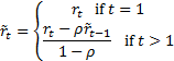
However, if we do this in practice we find that there are
second order effects that mean that estimating as above
still leaves some residual autocorrelation:
|
Period
|
(logged
returns of B)
|
(first
pass)
|
|
1
|
0.0487902
|
0.0487902
|
|
2
|
-0.1743534
|
-0.2611119
|
|
3
|
-0.1255632
|
-0.0728617
|
|
4
|
-0.0304592
|
-0.0139731
|
|
5
|
-0.0976128
|
-0.1301320
|
|
6
|
-0.0010005
|
0.0492060
|
|
7
|
-0.0801260
|
-0.1304104
|
|
8
|
0.0276152
|
0.0890558
|
|
9
|
0.1231022
|
0.1363395
|
|
10
|
0.0148886
|
-0.0323317
|
|
11
|
-0.1109316
|
-0.1414913
|
|
12
|
0.1106465
|
0.2086780
|
|
13
|
0.1646666
|
0.1475549
|
|
14
|
0.0925792
|
0.0712046
|
|
15
|
0.0797350
|
0.0830516
|
|
16
|
-0.0650720
|
-0.1226626
|
|
17
|
-0.0812101
|
-0.0650933
|
|
18
|
-0.0232686
|
-0.0070071
|
|
19
|
0.0525925
|
0.0757649
|
|
20
|
0.0276152
|
0.0088945
|
|
|
|
|
|
Variance (=)
|
0.0085758
|
0.0138041
|
|
Covariance (=)
|
0.0028964
|
0.0007054
|
|
Ratio (=)
|
0.3377457
|
0.0511003
|
|
Estimated
|
0.2799546
|
|
Better, therefore, is to use a root search algorithm in
which we explicitly search for the (ideally
between 0 and 0.5) for which has zero
autocorrelation. This can be done using the Nematrian MnDesmooth_AR1 or MnDesmooth_AR1_rho
functions (the former returns the desmoothed series, the latter returns the
value of for which
has zero
autocorrelation). Given the form of the problem given here, these provide the
following de-smoothed series (with rho equal to 0.31094682):
|
Period
|
(logged
returns of B)
|
(de-smoothed)
|
|
1
|
0.0487902
|
0.0487902
|
|
2
|
-0.1743534
|
-0.2750507
|
|
3
|
-0.1255632
|
-0.05810445
|
|
4
|
-0.0304592
|
-0.01798381
|
|
5
|
-0.0976128
|
-0.13354672
|
|
6
|
-0.0010005
|
0.05881321
|
|
7
|
-0.0801260
|
-0.14282465
|
|
8
|
0.0276152
|
0.10452905
|
|
9
|
0.1231022
|
0.13148365
|
|
10
|
0.0148886
|
-0.03772687
|
|
11
|
-0.1109316
|
-0.14396646
|
|
12
|
0.1106465
|
0.22554488
|
|
13
|
0.1646666
|
0.13719425
|
|
14
|
0.0925792
|
0.07244591
|
|
15
|
0.0797350
|
0.08302433
|
|
16
|
-0.0650720
|
-0.13190296
|
|
17
|
-0.0812101
|
-0.05833410
|
|
18
|
-0.0232686
|
-0.00744471
|
|
19
|
0.0525925
|
0.07968530
|
|
20
|
0.0276152
|
0.00411769
|
|
|
|
|
|
Variance (=)
|
0.0085758
|
0.01487681
|
|
Covariance (=)
|
0.0028964
|
0
|
|
Ratio (=)
|
0.3377457
|
0
|
Note:
(a) In
general de-smoothing increases the variance of the return series being
analysed. Here it has gone from 0.0926 to 0.1219.
(b) Whilst
the problem would usually be stated as shown, it perhaps makes more sense not
to make the arbitrary implicit assumption that the smoothing is around a mean
of zero, but around some mean (that is, for example, estimated from the data),
i.e. as if the model was  .
.
(c) We
might not necessarily want to give equal weight to each observation. This is
possible using the Nematrian MnWeightedDesmooth_AR1
and MnWeightedDesmooth_AR1_rho
functions.
NAVIGATION LINKS
Contents | Prev | Next | Question