Moments of a binomial loss distribution
[this page | pdf | back links]
Suppose a portfolio has  equally-sized
exposures. Each one is independent and has a probability
equally-sized
exposures. Each one is independent and has a probability  of
creating a unit loss (and a probability
of
creating a unit loss (and a probability  of
creating a zero loss), with the same
for each exposure, meaning that the portfolio loss,
of
creating a zero loss), with the same
for each exposure, meaning that the portfolio loss,  ,
is distributed according to a binomial distribution,
i.e.:
,
is distributed according to a binomial distribution,
i.e.:

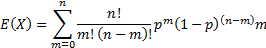
The mean and the variance of the portfolio loss distribution
can be found as follows. We note that:

The mean of the loss distribution is given by:

Likewise:


The variance of the loss distribution is:


Thus binomial distribution has mean  and
variance
and
variance  .
.
As  , the
Central Limit Theorem CLT implies that the binomial distribution tends to a normal distribution
with the same mean and variance, i.e. to
, the
Central Limit Theorem CLT implies that the binomial distribution tends to a normal distribution
with the same mean and variance, i.e. to  where
where  is the
cumulative normal distribution.
is the
cumulative normal distribution.