Enterprise Risk Management Formula Book
9. Risk measures
[this page | pdf | back links]
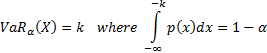
9.1 Value-at-Risk (VaR)
If  is a (continuous)
random variable (e.g. an outcome) with pdf
is a (continuous)
random variable (e.g. an outcome) with pdf  then the Value-at-Risk at
confidence level
then the Value-at-Risk at
confidence level  (e.g. 95%, 99%,
99.5%) is defined as:
(e.g. 95%, 99%,
99.5%) is defined as:
If has cdf  with an inverse
cdf, i.e. quantile function
with an inverse
cdf, i.e. quantile function  then
then 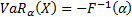 . Sometimes signs
are inverted and and
. Sometimes signs
are inverted and and  are
swapped around when defining
are
swapped around when defining  .
.
The relative VaR of relative
 , e.g. of an active
equity portfolio versus a benchmark portfolio is usually taken to mean the VaR
of the random variable
, e.g. of an active
equity portfolio versus a benchmark portfolio is usually taken to mean the VaR
of the random variable  . However, for
relative returns there are several alternative ways in which we can define the
equivalent of
. However, for
relative returns there are several alternative ways in which we can define the
equivalent of  , see definition of
tracking error.
, see definition of
tracking error.
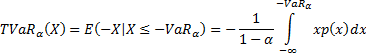
9.2 Tail Value-at-Risk (TVaR)
The Tail
Value-at-Risk (also called the conditional Value-at-Risk, CVaR) is
generally defined as the value of the loss conditional on it being worse than
the VaR at confidence level , so is defined as:
A coherent risk measure is one that satisfies subadditivity,
monotonicity, homogeneity and translational invariance. If
losses follow a continuous probability distribution then TVAR is a coherent
risk measure.
Occasionally TVaR (less commonly CVaR) is ascribed the same
meaning as expected shortfall, in which case the  factor is ignored,
or is defined relative to some specific limit
factor is ignored,
or is defined relative to some specific limit  that
in effect defines the to be used in the
above formula.
that
in effect defines the to be used in the
above formula.
9.3 Expected shortfall (ES)
The expected
shortfall, ES, and expected policyholder deficit, EPD are usually defined
as follows:
Expected policyholder deficit:
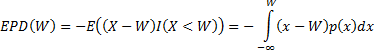
where  and
and  is
often but not always the policyholder wealth
is
often but not always the policyholder wealth
Expected shortfall:
Or more generally the expected shortfall below some trigger
level  is
is 
Sometimes expected shortfall is ascribed the same meaning as
is given above for TVaR.
9.4 Expected worst outcome (EWO)
The expected value of the worst outcome in  (non-overlapping)
observations is:
(non-overlapping)
observations is:

where the integral is -dimensional,  and the joint
distribution
and the joint
distribution  involves independent
marginal distributions each with pdf . This type of risk
measure can also be extended to, say,
involves independent
marginal distributions each with pdf . This type of risk
measure can also be extended to, say,  ’th worst outcome,
  with
with
 as defined above
being the special case where
as defined above
being the special case where  .
.
9.5 Tracking error (TE)
If is a random
variable (e.g. a portfolio return) with (assumed forward looking) pdf then its ex-ante
tracking error (if it exists) is  where
where

Nearly always is here the
relative return of a portfolio  of exposures versus
a benchmark portfolio
of exposures versus
a benchmark portfolio  and the tracking
error is then normally expressed as a percentage of the total portfolio value.
The tracking error of
and the tracking
error is then normally expressed as a percentage of the total portfolio value.
The tracking error of  versus
  is then
  (more precisely,
  for a time period
indexed by
for a time period
indexed by  ) where if the
future returns on the
) where if the
future returns on the  ’th instrument
during this are
’th instrument
during this are  and relative
returns are calculated arithmetically (i.e. using an arithmetic difference):
and relative
returns are calculated arithmetically (i.e. using an arithmetic difference):

where  is the vector of
active positions.
is the vector of
active positions.
If the  have covariance
matrix
have covariance
matrix  with elements
  then
then  .
.
However, returns compound rather than add through time so
for non-infinitesimal time period lengths there are alternative and potentially
preferable ways of defining relative returns, including (if we are trying to
calculate the return  relative to
  , each expressed as
fractions) using geometric relative returns, i.e.
, each expressed as
fractions) using geometric relative returns, i.e.  , or logarithmic
relative returns, i.e.
, or logarithmic
relative returns, i.e.  rather than
arithmetic relative returns
rather than
arithmetic relative returns  .
.
If a factor structure is assumed for the then this normally
involves assuming that:
where  is the exposure
(beta) of the ’th instrument to
the
is the exposure
(beta) of the ’th instrument to
the  ’th factor and
  are residual
(idiosyncratic) components.
are residual
(idiosyncratic) components.
A portfolio described by a vector of (active) weights then has an
expected return of  and an (expected)
future tracking error as follows, where
and an (expected)
future tracking error as follows, where  is the matrix
formed by and
is the matrix
formed by and  is the covariance
matrix between the factors
is the covariance
matrix between the factors


If  is the length of
time (time horizon) to which the ex-ante tracking error relates and returns in
individual time periods of length are assumed to be
independent of each other then (assuming e.g. we measure returns
logarithmically and that the portfolio and benchmark remain unchanged through
time) we can apply the square-root of time adjustment to derive ex ante
tracking errors applicable to different time periods, i.e.:
is the length of
time (time horizon) to which the ex-ante tracking error relates and returns in
individual time periods of length are assumed to be
independent of each other then (assuming e.g. we measure returns
logarithmically and that the portfolio and benchmark remain unchanged through
time) we can apply the square-root of time adjustment to derive ex ante
tracking errors applicable to different time periods, i.e.:

A portfolio’s ex-post tracking error is derived from
past observed values of its returns and might then be either a sample standard
deviation or (perhaps less accurately, but slightly lower) the corresponding
‘population’ standard deviation.
9.6 Drawdown
If a portfolio has exhibited past returns  over the previous time
periods (which could be days, weeks, months, years etc., where
over the previous time
periods (which could be days, weeks, months, years etc., where  is
earlier than
is
earlier than  etc.) then the
portfolio’s drawdown at time is usually defined
to be
etc.) then the
portfolio’s drawdown at time is usually defined
to be  (if negative). Its maximum
drawdown is usually defined as
(if negative). Its maximum
drawdown is usually defined as  (if negative). Its cumulative
maximum drawdown (i.e. peak-to-trough) at time is
usually defined by creating an index
(if negative). Its cumulative
maximum drawdown (i.e. peak-to-trough) at time is
usually defined by creating an index  such that
 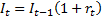 and then
determining at time the maximum of
and then
determining at time the maximum of 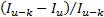 for all
  and
and
 .
.
9.7 Marginal VaR
The overall outcome of a portfolio of exposures containing a
(constant) amount  of exposure to the ’th
risk where each risk involves an random outcome
of exposure to the ’th
risk where each risk involves an random outcome  (technically is the value
ascribed to the random outcome) is
(technically is the value
ascribed to the random outcome) is  . Strictly speaking
combining exposures in this manner requires that the way in which we ascribe a
financial value to an outcome satisfies the axioms of uniqueness, additivity
and scalability, i.e. that
. Strictly speaking
combining exposures in this manner requires that the way in which we ascribe a
financial value to an outcome satisfies the axioms of uniqueness, additivity
and scalability, i.e. that  , the value we
ascribe to an outcome should be unique and should satisfy
, the value we
ascribe to an outcome should be unique and should satisfy  .
.
The VaR of such a portfolio with confidence level is
 .
.
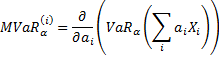
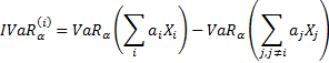
The marginal VaR with confidence level of
the ’th exposure in such
a portfolio is:
The contribution to overall VaR of the ’th
exposure is then  .
.
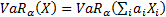
If the outcomes are Gaussian (i.e. multivariate normal, say  exposures
with
exposures
with 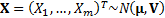 then
then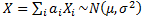 where:
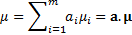
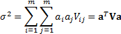
Here  and
and  . Given the
properties of the normal distribution
. Given the
properties of the normal distribution

As tracking error is a special case of VaR (with assumed
normal underlying distribution and  ,
,  ) we can likewise
define the marginal tracking error and contribution to tracking error from an
individual exposure.
) we can likewise
define the marginal tracking error and contribution to tracking error from an
individual exposure.
9.8 Incremental VaR
The incremental VaR with confidence level of
the ’th exposure in such
a portfolio is:
9.9 Estimating VaR
If the observations are normally distributed then  may be estimated
approximately in a parametric manner using
may be estimated
approximately in a parametric manner using 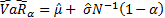 . Alternatively it
can be estimated (approximately) in a non-parametric manner (if the data does
not exhibit temporal dependencies) by taking the observations
. Alternatively it
can be estimated (approximately) in a non-parametric manner (if the data does
not exhibit temporal dependencies) by taking the observations  , say, reordering
them so that
, say, reordering
them so that  , say, identifying
the
, say, identifying
the  ’th order statistic,
where is an integer
between 1 and , and estimating the
VaR using the
’th order statistic,
where is an integer
between 1 and , and estimating the
VaR using the  ’th order statistic
where
’th order statistic
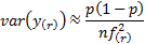
where  . Using a binomial
distribution, the variance of the ’th order statistic
is approximately as follows (where
. Using a binomial
distribution, the variance of the ’th order statistic
is approximately as follows (where  is the pdf at
  and
and  is
the probability of outcome) meaning that estimating the standard error of this
non-parametric statistic requires us to estimate :
is
the probability of outcome) meaning that estimating the standard error of this
non-parametric statistic requires us to estimate :
NAVIGATION LINKS
Contents | Prev | Next