Deriving the Black-Scholes Option Pricing
Formulae using Ito (stochastic) calculus and partial differential equations
[this page | pdf | references | back links]
The following partial differential equation is satisfied by
the price of any derivative on  , given the assumptions
underlying the Black-Scholes world:
, given the assumptions
underlying the Black-Scholes world:
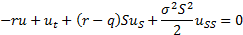
This partial differential equation is a second-order, linear
partial differential equation of the parabolic type. This type of
equation is the same as used by physicists to describe diffusion of heat. For
this reason, Gauss-Weiner or Brownian processes are also often commonly called diffusion
processes.
If  ,
,  and
and  are
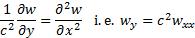
constant then we can solve it by transforming it into a standard form which
others have previously solved, namely (for some constant
are
constant then we can solve it by transforming it into a standard form which
others have previously solved, namely (for some constant  ):
):
This can be achieved by replacing  by
by  where
where
 (as long as is
constant) and by making the following double transformation (assuming that , and are
constant):
(as long as is
constant) and by making the following double transformation (assuming that , and are
constant):
This transformation removes one of the terms in the partial
differential equation:

The partial differential equation then simplifies to  , with
  . Prices of different
derivatives all satisfy this equation and are differentiated by the imposition
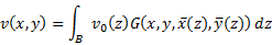
of different boundary conditions. A common tool for solving partial
differential equations subject to such boundary conditions is the use of Green’s
functions. This expresses the solution to a partial differential equation
given a general boundary condition applicable at some boundary
. Prices of different
derivatives all satisfy this equation and are differentiated by the imposition
of different boundary conditions. A common tool for solving partial
differential equations subject to such boundary conditions is the use of Green’s
functions. This expresses the solution to a partial differential equation
given a general boundary condition applicable at some boundary  , formed say by the
curve
, formed say by the
curve 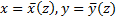 , as an expression of
the following form, in which
, as an expression of
the following form, in which  is called the Green’s
function for that partial differential equation:
is called the Green’s
function for that partial differential equation:
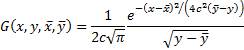
The Green’s function for where is
constant is:
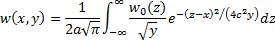
If the boundary condition is expressed as 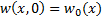 at
at  , where
  is continuous and
bounded for all
is continuous and
bounded for all  , then the solution is:
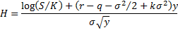
For a European call option, with strike price  , we
have, after making the substitutions described above,
, we
have, after making the substitutions described above,  . After some further
substitutions we find that this implies that:
. After some further
substitutions we find that this implies that:

where:

Substituting  and
and  into the formula for
  recovers the
Black-Scholes formulae, e.g. for a call option:
recovers the
Black-Scholes formulae, e.g. for a call option:

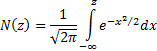
Where
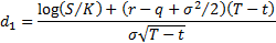
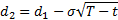
and  is the cumulative
Normal distribution function, i.e.
is the cumulative
Normal distribution function, i.e.