Stable Distributions
4. The Generalised Central Limit Theorem
[this page | pdf | references | back links]
Return
to Abstract and Contents
Next page
4.1 The two main reasons why stable laws are
commonly proposed for modelling return series are:
(a) The Generalised
Central Limit Theorem. This states that the only possible non-trivial limit
of normalised sums of independent identically distributed terms is stable; and
(b) Empirical. Many
large data sets exhibit fat tails (and skewness), and stable distributions form
a convenient family of distributions that can cater for such features (with
choice of  and
and  allowing
different levels of fat-tailed-ness or skewness to be accommodated).
allowing
different levels of fat-tailed-ness or skewness to be accommodated).
We focus below on the former, since there are other families
of distributions that can be parameterised in ways that can fit different
levels of fat-tailed-ness or skewness, including ones simpler to handle
analytically such as ones with quantile-quantile plots versus the Normal
distribution that are polynomials rather than straight lines, see e.g. Kemp (2009).
4.2 The classical Central Limit Theorem states that
the normalised sum of independent, identically distributed random variables
converges to a Normal distribution. The Generalised Central Limit Theorem shows
that if the finite variance assumption is dropped then the only possible
resulting limiting distribution is a stable one as defined above. Let  be
a sequence of independent, identically distributed random variables. Then there
exist constants
be
a sequence of independent, identically distributed random variables. Then there
exist constants  and
and
 and
a non-degenerate random variable
and
a non-degenerate random variable  with
with
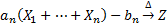
if and only if is stable (here  means
tends as
means
tends as  to the given
distributional form).
to the given
distributional form).
4.3 A random variable  is
said to be in the domain of attraction of if
there exist constants and
such
that the equation in Section 4.2 holds when are
independent identically distributed copies of . The
Generalised Central Limit Theorem thus shows that the only possible
distributions with a domain of attraction are stable distributions as described
above. Distributions within a given domain of attraction are characterised in
terms of tail probabilities. If is a random variable with
is
said to be in the domain of attraction of if
there exist constants and
such
that the equation in Section 4.2 holds when are
independent identically distributed copies of . The
Generalised Central Limit Theorem thus shows that the only possible
distributions with a domain of attraction are stable distributions as described
above. Distributions within a given domain of attraction are characterised in
terms of tail probabilities. If is a random variable with
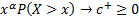 and
and 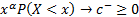 with
with  for
some
for
some  as
as  then is in
the domain of attraction of an -stable law.
then is in
the domain of attraction of an -stable law.  must
then be of the form
must
then be of the form 
NAVIGATION LINKS
Contents | Prev | Next