Risk Attribution
1. Introduction
[this page | pdf | references | back links]
Return
to Abstract and Contents
Next page
1.1 Traditionally, risk attribution (if the risk
model is characterised by a covariance matrix) proceeds as follows. We assume
that there are n different instruments in the universe in question. We
assume that the portfolio and benchmark weights can be represented by vectors  and
and  respectively. The
active positions are then
respectively. The
active positions are then  . If the risk model is
characterised in the parsimonious manner involving a factor covariance matrix,
. If the risk model is
characterised in the parsimonious manner involving a factor covariance matrix,  , and a sparce
idiosyncratic matrix,
, and a sparce
idiosyncratic matrix,  , e.g. as described in
Kemp (2009), then
, e.g. as described in
Kemp (2009), then  . The matrix describing
the covariance structure between factors, i.e. corresponds to a projection
of an n dimensional space onto a smaller m dimensional space.
. The matrix describing
the covariance structure between factors, i.e. corresponds to a projection
of an n dimensional space onto a smaller m dimensional space.
1.2 Factors might be further grouped into one of,
say,  different factor types,
using what we might call a factor classification,
different factor types,
using what we might call a factor classification,
 , i.e. a
  projection
matrix that has the property that each underlying factor is apportioned across
one or more ‘super’ factor types. By apportioned we mean that if
projection
matrix that has the property that each underlying factor is apportioned across
one or more ‘super’ factor types. By apportioned we mean that if  corresponds to the
exposure that the j’th factor has to the k’th factor type then
the sum of these exposures for any given factor is unity, i.e.
corresponds to the
exposure that the j’th factor has to the k’th factor type then
the sum of these exposures for any given factor is unity, i.e.  .
.
1.3 Usually such a factor classification (at least
in equity-land) would involve unit disjoint elements, i.e. each factor would be
associated with a single ‘super’ factor type. For example, equity sector
classification structures are usually hierarchical, so each industry subgroup
is part of a (single) overall market sector. More generally, factors might be
apportioned across more than one factor type. The aggregate (relative) exposure
to the different factor types is then, in matrix algebra terms, equal to  .
.
1.4 To decompose (or ‘attribute’) the tracking
error into its main contributors it is usual to decompose the tracking error,  , in the manner
described in Kemp
(2005), Kemp
(2009) or Heywood,
Marsland and Morrison (2003), i.e. in line with partial differentials
(scaled if necessary by a uniform factor so that the total adds up to the total
tracking error). For example, if the aim is to identify the risk contribution
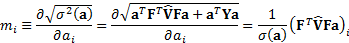
coming from each individual security then we might calculate the marginal
contribution to tracking error,
, in the manner
described in Kemp
(2005), Kemp
(2009) or Heywood,
Marsland and Morrison (2003), i.e. in line with partial differentials
(scaled if necessary by a uniform factor so that the total adds up to the total
tracking error). For example, if the aim is to identify the risk contribution
coming from each individual security then we might calculate the marginal
contribution to tracking error,
 , and the contribution
to tracking error,
, and the contribution
to tracking error,  , from the i’th
instrument as follows:
, from the i’th
instrument as follows:

1.5 This has  , so the sum of the
individual contributions assigned to each instrument is the total tracking
error of the portfolio. Simetimes writers instead focus on decomposing the
variance rather than the standard deviation. However the answers are the same
up to a scaling factor. This is to be expected since for any two functions,
, so the sum of the
individual contributions assigned to each instrument is the total tracking
error of the portfolio. Simetimes writers instead focus on decomposing the
variance rather than the standard deviation. However the answers are the same
up to a scaling factor. This is to be expected since for any two functions,  and
and  with
first differentials
with
first differentials  and
and  we have
  , i.e. the vector of
partial differentials is the same, up to a scaling factor for all functions of
same underlying risk measure. Variance and standard deviation in this context
relate to the ‘same’ underlying risk measure, since variance is the square of
standard deviation.
, i.e. the vector of
partial differentials is the same, up to a scaling factor for all functions of
same underlying risk measure. Variance and standard deviation in this context
relate to the ‘same’ underlying risk measure, since variance is the square of
standard deviation.
1.6 We can group the in whatever manner we
like, as long as each relative position is assigned to a unique grouping or if
it is split across several groupings then in aggregate a unit contribution
arises from it.
1.7 For example, suppose that we have a
classification described by the  matrix
  with elements
  being the contribution
that the i’th instrument makes to the q’th classification. As it
is a classification it needs to satisfy
being the contribution
that the i’th instrument makes to the q’th classification. As it
is a classification it needs to satisfy  so
so 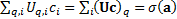 , i.e. grouping in this
manner is equivalent to calculating
, i.e. grouping in this
manner is equivalent to calculating  where
where  .
.
1.8 A special case of such a classification would
be to calculate the contribution to risk from a given issuer (rather than a
given instrument), e.g. for a bond portfolio, where would be 1 if issue  is
issued by issuer
is
issued by issuer  and 0 otherwise.
1.9 The above approach calculates a single overall
contribution to tracking error for each individual instrument (and then if
necessary groups them). For bond risk analysis (and also in some instances for
equity risk analysis) it may be more illuminating to subdivide these instrument
specific contributions into several different sub-elements, each one relating
to a given factor type. These factor types might be, say, currency, interest
rate (duration), credit, sector, other factors and idiosyncratic.
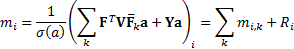
1.10 To do this we need to subdivide  into several different
elements, which cumulatively add up to , each relating to a
different factor type, i.e. we define, say,
into several different
elements, which cumulatively add up to , each relating to a
different factor type, i.e. we define, say,  each of which are
  matrices,
which have the property that the
matrices,
which have the property that the  ’th element of
  is calculated as
  for a given factor
classification . The sum of the for all
for a given factor
classification . The sum of the for all  is
then
is
then  . We can then decompose
the marginal contributions to tracking error into the following, where
. We can then decompose
the marginal contributions to tracking error into the following, where  and
and  :
:
NAVIGATION LINKS
Contents | Prev | Next