Blending Independent Components and
Principal Components Analysis
3.1 Characteristics of PCA
[this page | pdf | references | back links]
Return to
Abstract and Contents
Next page
3.1 Characteristics
of PCA
Earlier, we noted some similarities between ICA and PCA but
also noted some differences. In particular, ICA focuses on ‘independence’,
‘non-Normality’ and ‘lack of complexity’ and assumes that source signals
exhibit these features, whereas PCA focuses merely on lack of correlatedness.
Indeed, PCA analysis will even ‘unmix’ pure Gaussian (i.e. normally
distributed) signals. Or rather, it will decompose multiple Gaussian output
signals into some presumed orthogonal Gaussian input signals, which can be
ordered with ones higher up the ordering explaining more of the variability in
the output signal ensemble than ones lower down the ordering.
PCA involves calculating the eigenvectors and eigenvalues of
the covariance matrix, i.e. the matrix of correlation coefficients between the
different signals. Usually, it would be assumed that the covariance matrix had
been calculated in a manner that gives equal weight to each data point.
However, this is not essential; we could equally use a computation approach in
which different weights were given to different data points, e.g. an
exponentially decaying weighting that gives greater weight to more recent
observations.
For  different
output signals
different
output signals  , with
covariance matrix,
, with
covariance matrix,  , between the
output signals, PCA searches for the (some possibly
degenerate) eigenvectors,
, between the
output signals, PCA searches for the (some possibly
degenerate) eigenvectors,  , satisfying
the following matrix equation for some scalar
, satisfying
the following matrix equation for some scalar  .
.

For a non-negative definite symmetric matrix (as should
be if it actually corresponds to a covariance matrix), the values
of are all
non-negative. We can therefore order the eigenvalues in descending order  . The
corresponding eigenvectors
. The
corresponding eigenvectors  are orthogonal
i.e. have
are orthogonal
i.e. have  if
if  and
are also typically normalised so that
and
are also typically normalised so that  (i.e. so that
they have ‘unit length’). For any ’s that are
equal, we need to choose a corresponding number of orthonormal eigenvectors
that span the relevant subspace.
(i.e. so that
they have ‘unit length’). For any ’s that are
equal, we need to choose a corresponding number of orthonormal eigenvectors
that span the relevant subspace.
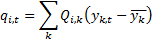
By we mean the
vector  such that the
signal corresponding to eigenvalue
such that the
signal corresponding to eigenvalue  is expressible
as:
is expressible
as:
If  is the matrix
with coefficients
is the matrix
with coefficients  then the
orthonomalisation convention adopted above means that
then the
orthonomalisation convention adopted above means that  where
where  is
the identity matrix. This means that
is
the identity matrix. This means that  and hence we
may also write the output signals as a linear combination of the eigenvector
signals as follows (in each case up to a constant value, since the covariances
do not depend on means of series):
and hence we
may also write the output signals as a linear combination of the eigenvector
signals as follows (in each case up to a constant value, since the covariances
do not depend on means of series):
Additionally, we have  if and
 if
if  .
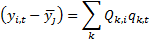
We also note that if
.
We also note that if  are the
coefficients of then each
individual is (here
assuming that we have been using ‘sample’ rather than ‘population’ values for
variances:
are the
coefficients of then each
individual is (here
assuming that we have been using ‘sample’ rather than ‘population’ values for
variances:
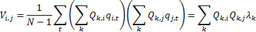
Hence the sum of the variances of each output signal, i.e.
the trace of the covariance matrix, satisfies:

We can interpret this as indicating that the aggregate
variability of the output signals (i.e. the sum of their individual
variabilities) is equal to the sum of the eigenvalues. Hence the larger the eigenvalue
the more the corresponding eigenvector signal ‘contributes’ to the aggregate
variability across the ensemble of possible output signals.
NAVIGATION LINKS
Contents | Prev | Next