Extreme Events – Specimen Question A.2.3(b)
– Answer/Hints
[this page | pdf | references | back links]
Return
to Question
Q. Prepare a (standardised) quantile-quantile
plot of the weighted data. Is it also suggestive of fat-tailed behaviour? Hint:
the ‘expected’ values for such plots need to bear in mind the weight given to
the observation in question.
We need to:
(a) Scale the
weights so that they add to unity
(b) Standardise the
observations, so that they have weighted mean equal to zero and weighted
(sample) standard deviation equal to unity
(c) Sort the data
(d) Work out the quantile
plots corresponding to each data point (e.g. assume the data point corresponds
to the cumulative (scaled) weight of smaller points plus one-half of the
(scaled) weight of the observation in question
(e) Identify standardised
inverse normal values corresponding to the quantile points in (d)
(f) Plot
‘observed’ vs ‘expected’, the latter being the values from (e)
Steps (a) and (b) give:
|
Period
|
Scaled Weight
|
Standardised Observation
|
|
1
|
0.0239245
|
-3.7746674
|
|
2
|
0.0256416
|
0.0229646
|
|
3
|
0.0274820
|
2.8477710
|
|
4
|
0.0294545
|
1.0055183
|
|
5
|
0.0315686
|
-0.1747424
|
|
6
|
0.0338343
|
0.0751858
|
|
7
|
0.0362627
|
-0.0689278
|
|
8
|
0.0388654
|
0.1401715
|
|
9
|
0.0416550
|
0.9325003
|
|
10
|
0.0446447
|
-1.6640468
|
|
11
|
0.0478490
|
0.1012191
|
|
12
|
0.0512833
|
0.1142167
|
|
13
|
0.0549640
|
-0.4974175
|
|
14
|
0.0589090
|
0.3714857
|
|
15
|
0.0631371
|
-0.5656546
|
|
16
|
0.0676687
|
-0.1482089
|
|
17
|
0.0725255
|
-0.9404055
|
|
18
|
0.0777309
|
0.8345045
|
|
19
|
0.0833099
|
0.4729935
|
|
20
|
0.0892893
|
0.2434824
|
Steps (c), (d) and (e) give:
|
Scaled Weight
|
Observation (i.e. ‘Observed’)
|
Quantile Point
|
‘Expected’
|
|
0.0239245
|
-3.7746674
|
0.0119622
|
-2.2583397
|
|
0.0446447
|
-1.6640468
|
0.0462468
|
-1.6823879
|
|
0.0725255
|
-0.9404055
|
0.1048319
|
-1.2544904
|
|
0.0631371
|
-0.5656546
|
0.1726632
|
-0.9436933
|
|
0.054964
|
-0.4974175
|
0.2317138
|
-0.7332146
|
|
0.0315686
|
-0.1747424
|
0.2749801
|
-0.5978199
|
|
0.0676687
|
-0.1482089
|
0.3245987
|
-0.4548775
|
|
0.0362627
|
-0.0689278
|
0.3765644
|
-0.3145165
|
|
0.0256416
|
0.0229646
|
0.4075166
|
-0.233938
|
|
0.0338343
|
0.0751858
|
0.4372545
|
-0.1579336
|
|
0.047849
|
0.1012191
|
0.4780962
|
-0.0549323
|
|
0.0512833
|
0.1142167
|
0.5276623
|
0.0693948
|
|
0.0388654
|
0.1401715
|
0.5727367
|
0.1833459
|
|
0.0892893
|
0.2434824
|
0.6368141
|
0.3499558
|
|
0.058909
|
0.3714857
|
0.7109132
|
0.5560546
|
|
0.0833099
|
0.4729935
|
0.7820227
|
0.7790426
|
|
0.0777309
|
0.8345045
|
0.8625431
|
1.0918164
|
|
0.041655
|
0.9325003
|
0.922236
|
1.4202738
|
|
0.0294545
|
1.0055183
|
0.9577907
|
1.7256048
|
|
0.027482
|
2.847771
|
0.986259
|
2.2046022
|
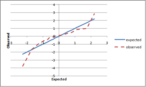
The following chart plots the observed vs expected values,
using Microsoft Excel. It is also suggestive of fat-tailed behaviour:
However, in practice it is easier to use the Nematrian
Charting facility, i.e. MnPlotWeightedStandardisedQQ
which can do all of these steps simultaneously.
NAVIGATION LINKS
Contents | Prev | Next | Question