Constrained Quadratic Optimisation: 2.
Solving the canonical problem
[this page | pdf | references | back links]
Return to
Abstract and Contents
Next
page
2. Solving the
canonical problem
We can solve the canonical
problem using a variant of the Simplex algorithm, as follows:
(a) We use the
method of Lagrange multipliers, where 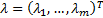 and
and 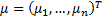 are the
Lagrange multipliers corresponding to the two sets of constraints
are the
Lagrange multipliers corresponding to the two sets of constraints  and
and  respectively.
(b) We introduce further
‘slack’ variables, 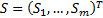 for the
constraints
for the
constraints  , i.e. we
define
, i.e. we
define  .
.
(c) Application of
the Kuhn-Tucker conditions then implies that the canonical problem can be
solved using a variant of the Simplex algorithm, using a Simplex ‘tableau’
(bearing in mind that  ) as follows,
see e.g. Taha
(1976):
) as follows,
see e.g. Taha
(1976):
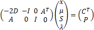
subject to  for
for  ,
,
 and
and  .
.
Loosely speaking, the algorithm works as follows:
(i) We
start with a feasible solution (i.e. a solution that satisfies all of the
constraints), which will be characterised by some value of  ;
;
(ii) We then identify
a methodical way of improving on (if
possible), whilst staying within the set of feasible solutions; and
(iii) We iterate (ii) until
we run out of ability to improve .
Conveniently, because of the convex nature of the feasible
solution set, the Simplex algorithm is in this case guaranteed to converge.
Moreover, because the loss function is quadratic and positive definite, it
converges to the global optimum and not just a local optimum.
The relative ease with which it is possible to solve
quadratic optimisation problems is one reason why quadratic utility functions
are so commonly used in quantitative finance, see Kemp (2010).
However, there is one complication. For the algorithm to
work properly we need to start with a ‘feasible’ solution – if we start with
one that isn’t feasible then the algorithm sometimes converges to a feasible
solution but sometimes it doesn’t. We do not necessarily end up with a feasible
solution merely by starting with  , since the
left hand side of the tableau then equates to zero, but the right hand side
doesn’t. What we therefore need to do is to add additional variables to create
a superset of the original optimisation problem for which it is easy to
identify a (basic) feasible solution, the additional variables being set up in
such a way that when we have converged on the solution to the superset problem
we will then either:
, since the
left hand side of the tableau then equates to zero, but the right hand side
doesn’t. What we therefore need to do is to add additional variables to create
a superset of the original optimisation problem for which it is easy to
identify a (basic) feasible solution, the additional variables being set up in
such a way that when we have converged on the solution to the superset problem
we will then either:
(1) Have reached a
feasible solution to the original problem, in which case we have the solution;
or
(2) We still have an
infeasible solution, in which case we can conclude that there was no feasible
solution to the original problem.
NAVIGATION LINKS
Contents | Prev | Next